
| 일 | 월 | 화 | 수 | 목 | 금 | 토 |
|---|---|---|---|---|---|---|
| 1 | 2 | 3 | ||||
| 4 | 5 | 6 | 7 | 8 | 9 | 10 |
| 11 | 12 | 13 | 14 | 15 | 16 | 17 |
| 18 | 19 | 20 | 21 | 22 | 23 | 24 |
| 25 | 26 | 27 | 28 | 29 | 30 | 31 |
- Machine Learning
- GPT
- prompt
- coursera
- 인공신경망
- Andrew Ng
- 프롬프트 엔지니어링
- bingai
- AI 트렌드
- ChatGPT
- AI
- Deep Learning
- Supervised Learning
- feature scaling
- 인공지능
- llama
- Regression
- learning algorithms
- 챗지피티
- 언어모델
- ML
- supervised ml
- 머신러닝
- feature engineering
- Unsupervised Learning
- 딥러닝
- LLM
- neural network
- Scikitlearn
- nlp
- Today
- Total
My Progress
[Supervised ML] Multiple linear regression - 4 본문
1. Intuition
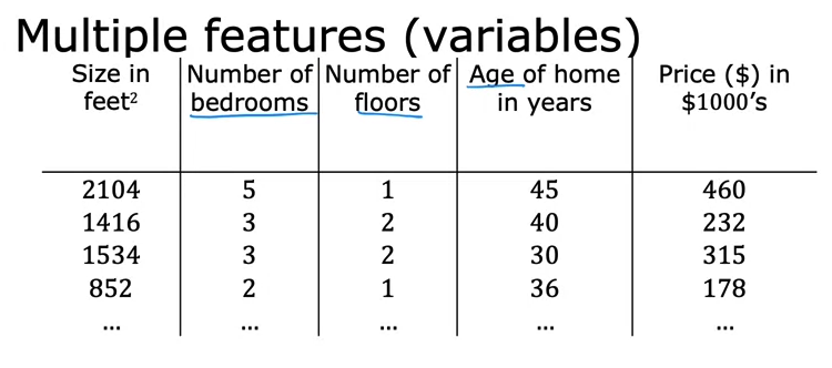
Instead of prediction house price with only the size of a house, we can use multiple features of a house to make a better prediction
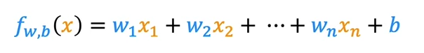
This is a standard notation for multiple linear regression
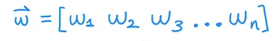
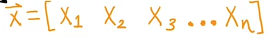
W and X can be represented in the form of vectors.
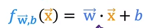
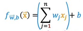
This is the other format of writing multiple linear regression equation.
Multiplication of vectors are called "Dot Product"
2. Vectorization
Def: Vectorization allows easier mathematical calculation among vectors
Without Vectorization:
Case 1:

f = w[0] * x[0] + w[1] * x[1] + w[2] * x[2] + b
Case 2:
f = 0
for j in range(0, n):
	f = f + w[j] * x[j]
f = f + b
With vectorization:
w = np.array([1.0, 2.5, -3.3])
b = 4
x = np.array([10, 20, 30])

f = np.dot(w, x) + b
Vectorization is much faster because np.dot() function uses parallel calculation, while other cases uses sequential calculation.
During parallel calculation, each w and x is calculated simultaneously.
Example - Gradient descent with vectorization
Without vectorization:
for j in range(0, 16):
	w[j] = w[j] - 0.1 * d[j]
With vectorization:
w = w - 0.1 * d
3. Gradient descent for multiple linear regression
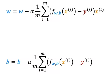
Gradient descent notation with one feature:
Gradient descent notation with multiple feature:
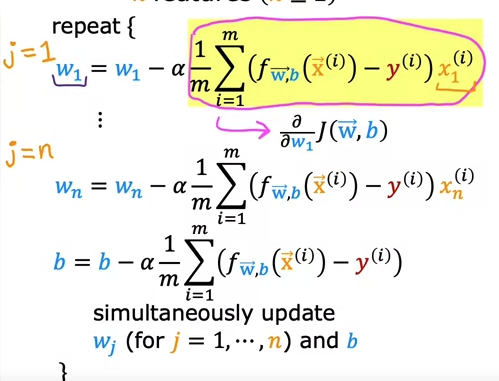
Since there are multiple w, every w has to be updated.
4. Code
4.1 Computing Cost for multiple linear regression
def compute_cost(X, y. w. b):
	#X: matrix of examples with multiple features

    m = X.shape[0]
    cost = 0.0
    for i in range(m):
    	f_wb_i = np.dot(X[i], w) + b
        cost = cost + (f_wb - y[i])**2
    cost = cost/(2*m)

    return cost
4.2.1 Gradient descent for multiple linear regression (Derivative)
def compute_gradient(X, y, w, b):

    m, n = X.shape
    dj_dw = np.zeros((n, ))
    dj_db = 0.

    for i in range(m):
    	err = (np.dot(X[i], w) + b) - y[i]
        for j in range(n)
        	dj_dw[j] = dj_dw[j] + err * X[i, j]
        dj_db = dj_db + err
    dj_dw = dj_dw/m
    dj_db = dj_db/m

    return dj_db, dj_dw
'AI > ML Specialization' 카테고리의 다른 글
| [Supervised ML] Gradient descent / Learning Rate - 6 (0) | 2023.07.28 |
|---|---|
| [Supervised ML] Feature scaling - 5 (0) | 2023.07.28 |
| [Supervised ML] Gradient Descent - 3 (0) | 2023.07.27 |
| [Supervised ML] Regression/ Cost function - 2 (0) | 2023.07.26 |
| [Supervised ML] Supervised/Unsupervised - 1 (0) | 2023.07.26 |


