
| 일 | 월 | 화 | 수 | 목 | 금 | 토 |
|---|---|---|---|---|---|---|
| 1 | ||||||
| 2 | 3 | 4 | 5 | 6 | 7 | 8 |
| 9 | 10 | 11 | 12 | 13 | 14 | 15 |
| 16 | 17 | 18 | 19 | 20 | 21 | 22 |
| 23 | 24 | 25 | 26 | 27 | 28 | 29 |
| 30 |
- ChatGPT
- learning algorithms
- 챗지피티
- coursera
- Deep Learning
- bingai
- feature scaling
- prompt
- Andrew Ng
- supervised ml
- Unsupervised Learning
- Supervised Learning
- llama
- 언어모델
- ML
- nlp
- 머신러닝
- GPT
- neural network
- Regression
- AI
- 인공신경망
- Scikitlearn
- AI 트렌드
- feature engineering
- 프롬프트 엔지니어링
- Machine Learning
- LLM
- 딥러닝
- 인공지능
- Today
- Total
My Progress
[Supervised ML] Cost function/Gradient descent for logistic regression - 9 본문
[Supervised ML] Cost function/Gradient descent for logistic regression - 9
ghwangbo 2023. 7. 31. 17:141. Cost function
1.1 Intuition
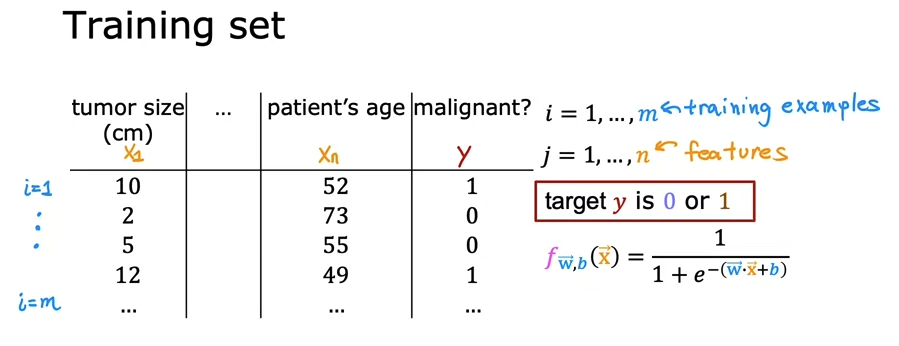
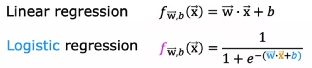
We use logistic regression / sigmoid function to estimate the data's label or category.
How do we choose w and b?
For linear regression, we used squared error cost.
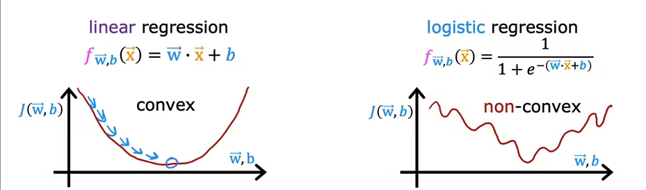
Linear regression is a convex form, so we could use standard gradient descent equation to figure out local minimum.
Since logistic regression is a non-convex form, it has multiple local minimum. Thus, we cannot use the standard cost function which is a mean squared error function.
1.2 Cost function
The graph intersects the x-axis when x is 1. In logistic function, we only get either 0 or 1 for the output. Therefore, we only care about the x-intercept.
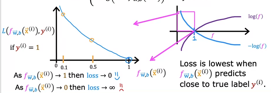
This is when the answer is 1. As our prediction approaches 1, the loss decreases.
However, when it's 0, the loss approaches infinity.
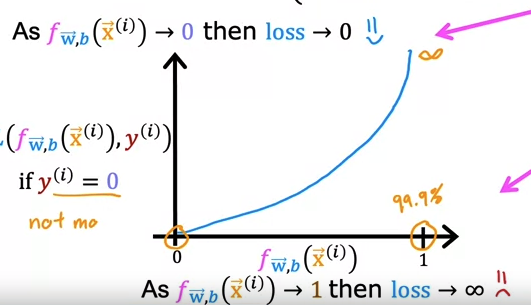
Image above shows when the output is 0. When our prediction is 0, the loss is 0.
When the prediction is 1, the loss approaches infinity.
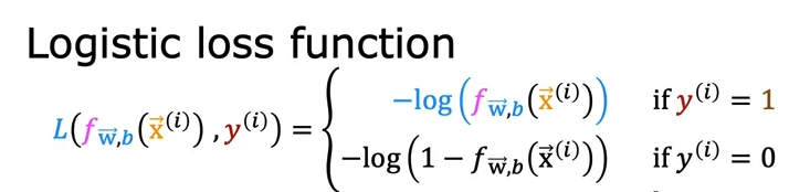
A key for cost function for logistic regression. We want to get a global minimum to find the most optimized w. However, squared error cost function yields multiple minimum. It makes us to use logarithmic cost function, which gives us 0 when the y equals to probability 0 or 1 we want.
1.3 Simplified cost function
Loss function:
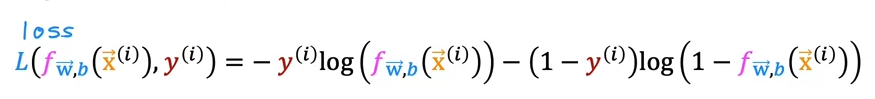
This function is identical function as 2 functions above.
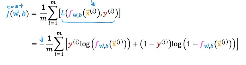
Using the loss function, we now can make the cost function to find the best w and b for machine learning model.
Negative sign in front was took out from the equation inside.
2. Gradient descent
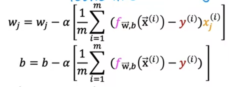
Gradient descent for logistic regression may look the same as the one for linear regression.
But f(x) is different for logistic regression.
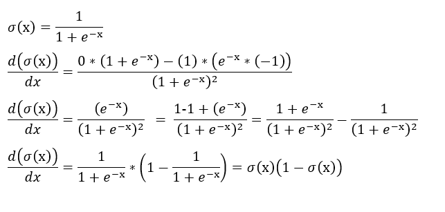
Interpretation
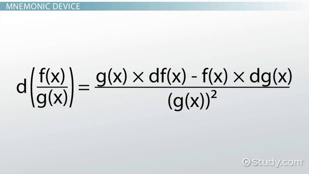
We first have to take the derivative of the logistic regression function in order to run gradient descent.
3. Code
Using logistic regression model from scikit learn
Fit the model
from sklearn.linear_model import LogisticRegression

lr_model = LogisticRegression()
lr_model.fit(X,y) #X and Y are datasets
Make Predictions
y_pred = lr_model.predict(X)

print("prediction on training set: ", y pred)
Calculate accuracy
print("Accuracy on training set: ", lr_model.score(X,y))'AI > ML Specialization' 카테고리의 다른 글
| [Supervised ML] Review - 11 (0) | 2023.08.03 |
|---|---|
| [Supervised ML] The problem of overfitting / Regularization - 10 (0) | 2023.08.01 |
| [Supervised ML] Classification with logistic regression - 8 (1) | 2023.07.30 |
| [Supervised ML] Feature Engineering - 7 (0) | 2023.07.28 |
| [Supervised ML] Gradient descent / Learning Rate - 6 (0) | 2023.07.28 |


